Learning Quantum Mechanics The Hard Way
John S. Bell in his landmark paper On The EPR Paradox considered the EPR experiment with a modification - Alice and Bob’s detectors are no longer oriented along the same axis. Alice detector is oriented along \(\vec{a}\) and Bob’s detector is oriented along \(\vec{b}\).
Question: What is the expected value of Alice’s spin \(\times\) Bob’s spin?
Bell solves it in one line. Or rather, he just gives the answer and leaves it to the reader to work it out:
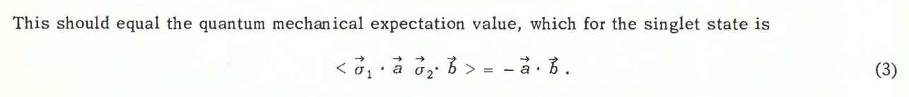
This problem also appears as Problem 4.55 in DJ Griffiths Introduction to Quantum Mechanics 2nd ed.
Working it out is not trivial for me. I actually had to use the sympy package in Python to work it out (the hard or poor man’s way).
Let’s get started. I won’t be showing the full code but bits and pieces of it. First, create the vector corresponding to the spin-singlet state i.e., \(\frac{1}{\sqrt{2}}(|01\rangle - |10\rangle)\):
psi = 1 / sympy.sqrt(2) * Matrix([[0],[1],[-1],[0]])Next, create the \(2 \times 2\) matrices corresponding to Alice and Bob. The matrices are identical except for the axes they use:
a1, a2, a3, b1, b2, b3 = sympy.symbols('a1 a2 a3 b1 b2 b3', real=True)
M_A = a1 * X + a2 * Y + a3 * Z
M_B = b1 * X + b2 * Y + b3 * Z
where X, Y, Z are the Pauli matrices. Now notice that psi is a \(4 \times 1\) vector but the matrices above are \(2 \times 2\). The \(4 \times 4\) matrix corresponding to Alice’s observable is given by \(I \otimes M_A\) and conversely the \(4 \times 4\) matrix corresponding to Bob’s observable is given by \(M_B \otimes I\) where \(I\) of course is the identity matrix.
We can calculate these matrices using the TensorProduct function (it takes arguments in “opposite” order):
Alice = TensorProduct(M_A, eye(2))
Bob   = TensorProduct(eye(2), M_B)
Now we write a function which will simulate Alice making a measurement on her qubit:
alice_measurements, alice_probabilities, psis = measure(psi, Alice)Writing the measure function is left as exercise and is key to solving the problem.
The measure function takes input the wavefunction psi and an observable (given by Alice in above).
Remember an observable is a Hermitian matrix. The function returns us 3 things:
-
an array of possible measurement outcomes. This is computed by computing the distinct eigenvalues of the input observable. In our case we will get only two distinct eigenvalues: \(+1\) and \(-1\).
-
an array of the respective probabilities of the outcomes.
-
an array containing the collapsed wavefunction in each case.
Next, we need to simulate Bob’s measurement for each possible outcome of Alice’s measurement (so we have a nested loop):
for i in range(0, len(alice_measurements)):
    alice_spin = alice_measurements[i]
    alice_prob = alice_probabilities[i]
    psi = psis[i]
    bob_measurements, bob_probabilities, bob_psis = measure(psi, Bob)
    for j in range(0, len(bob_measurements)):
        bob_spin = bob_measurements[j]
        bob_prob = bob_probabilities[j]
        spin_product.append(alice_spin * bob_spin)
        probabilities.append(alice_prob * bob_prob)
The final answer i.e., expected value of Alice’s spin \(\times\) Bob’s spin is given by:
for i in range(0, len(spin_product)):
    expectation += spin_product[i] * probabilities[i]

sympy.pprint(expectation)
Running this does not give the simple \(- \vec{a} \cdot \vec{b}\). Instead I get a monstrous expression. I tried simplifying it using the simplify function but it didn’t help.
To check I didn’t have a bug in my code, I evaluated the expression (i.e., compute a numerical value) using the n() or N function in sympy and that did give correct result.
So I don’t think there was bug in the code; just that sympy is not able to simplify the expression.
The hard way does it using basic principles. And the algorithm can be generalized to any case. But its infeasible to do calculations like this by hand. How did Bell calculate it by hand? There ought to be a shortcut.
The Smart Way
Now that we have solved the problem the hard way, let’s see how to solve it the smart way. It turns out the answer to the problem is given by the expected value of the observable formed by \(M_B \otimes M_A\) (or vice-versa). i.e.,
\begin{equation} \langle \psi | M_B \otimes M_A | \psi \rangle = - \vec{a} \cdot \vec{b} \end{equation}
where \(\psi\) once again is given by \(\frac{1}{\sqrt{2}}(|01\rangle - |10\rangle)\) or \( \begin{pmatrix} 0 \\ \frac{\sqrt{2}}{2} \\ -\frac{\sqrt{2}}{2} \\ 0 \end{pmatrix} \) and that is what Bell is referring to in his paper.
But why is it like that? First, we - or at least I - know that the expected value of an observable \(M\) (sometimes also referred to as operator) is indeed given by \(\langle \psi | M | \psi \rangle\). The proof of this can be found in Nielsen and Chuang, equation 2.113 p. 88. Now let’s look at \(M_B \otimes M_A\):
\begin{equation} \label{eq1} \begin{split} M_B \otimes M_A & = (b_1 uu^T + b_2 vv^T) \otimes (a_1 qq^T + a_2 rr^T) \\ & = a_1 b_1 uu^T \otimes qq^T + a_2 b_1 uu^T \otimes rr^T + a_1 b_2 vv^T \otimes qq^T + a_2 b_2 vv^T \otimes rr^T \\ & = a_1 b_1 (u \otimes q)(u \otimes q)^T + a_2 b_1 (u \otimes r)(u \otimes r)^T + a_1 b_2 (v \otimes q)(v \otimes q)^T + a_2 b_2 (v \otimes r)(v \otimes r)^T \end{split} \end{equation}
The math above itself is not obvious. \(a_1, a_2\) are eigenvalues of \(M_A\). Similarly \(b_1, b_2\) are eigenvalues of \(M_B\). \(q, r\) are eigenvectors of \(M_A\) and \(u, v\) are eigenvectors of \(M_B\). The first line follows from the property of eigendecomposition of a matrix and is used often in Nielsen and Chuang. See box 2.2 p. 72 for example. To get the second line, prove that the tensor product distributes over addition. Don’t take it for granted. See equations 2.43 and 2.44 p. 73 in Nielsen & Chuang. To get the third line is very difficult for me so I posted it as a question on SE. It relies on two properties (don’t take them for granted, prove them):
\begin{equation} \label{eq2} \begin{split} (u \otimes q)^T & = u^T \otimes q^T (\textrm{eq. 2.53 p.74 Nielsen & Chuang}) \\ (u \otimes q)(u^T \otimes q^T) & = uu^T \otimes qq^T (\textrm{mixed product property}) \end{split} \end{equation}
Now we have written \(M_B \otimes M_A\) as an eigendecomposition and can see that its eigenvalues are nothing but the product of the eigenvalues of Alice and Bob’s matrices. And we are done. QED.
All that is left is to compute \(\langle \psi | M_B \otimes M_A | \psi \rangle\) and that is something that can be done by hand - not easy for me so I am going to use
sympy again.
>>> t = psi.H * TensorProduct(M_A, M_B) * psi
>>> t
⎡   ⎛  √2⋅a₃⋅b₃   √2⋅(a₁ + ⅈ⋅a₂)⋅(b₁ - ⅈ⋅b₂)⎞      ⎛√2⋅a₃⋅b₃   √2⋅(a₁ - ⅈ⋅a₂)⋅(b₁ + ⅈ⋅b₂)⎞⎤
⎢√2⋅⎜- ──────── - ──────────────────────────⎟   √2⋅⎜──────── + ──────────────────────────⎟⎥
⎢   ⎝     2                   2             ⎠      ⎝   2                   2             ⎠⎥
⎢──────────────────────────────────────────── - ──────────────────────────────────────────⎥
⎣                     2                                             2                     ⎦
>>> t.simplify()
>>> t
[-a₁⋅b₁ - a₂⋅b₂ - a₃⋅b₃]
Probability that qubits are the same
Note that the expected value of the product of spins is different from the probability that the spins are equal. This probability is used in e.g., this video (Fast Forward to 4:30 if you like). Also see section 2.2 on p.21 in this pdf.
which gives:
which is the formula in that video - or is it? The formula in the video is \(\cos^2 \theta\). Another problem is that \(E[s_a \times s_b]\) is equal to \(-\cos \theta\) (refer Bell equation again if you like) and not \(+ \cos \theta\). What gives? The \(\Psi\) we have used is different from the \(\Psi\) used in the video. In the video he is using:
and if we do that:
t = psi.H * TensorProduct(M_A, M_B) * psi
gives:
>>> t.simplify()
>>> t
[a₁⋅b₁ - a₂⋅b₂ + a₃⋅b₃]
This formula is also worked out in this article. But this also is not \(+ \cos \theta\). What gives now? Well the answer is this: consider what happens to the state \(\frac{1}{\sqrt 2}|00\rangle + \frac{1}{\sqrt 2}|11\rangle\) when it is subjected to an arbitrary unitary transform with bases \(u\) and \(u^ \perp\). Thus, let:
giving:
Here \(\alpha^2\) is \(\alpha^2\). It is not \(|\alpha|^2\). For \(|11\rangle\) we get:
and so in the new basis:
and this is equal to \(|uu\rangle + |u^\perp u^\perp \rangle\) (an assumption Vazirani is making in his video if you analyze his logic carefully) only if:
thus the tranform cannot be arbitrary. It has to be a rotation. In other words, \(|\Phi^+\rangle\) is invariant to a rotation but not otherwise. This is actually called out in this article as well. At the very top of his slide Vazirani does say in bold Rotational Invariance of the Bell State. So he is not considering any arbitrary transform. He is only considering rotational transforms and the axes \(u, u^\perp, v, v^\perp\) lie in the \(xz\) plane i.e., the \(y\) component is zero. When that is the case, then a₁⋅b₁ - a₂⋅b₂ + a₃⋅b₃ reduces to a₁⋅b₁ + a₃⋅b₃ and is equal to \(\cos \theta\). There is still a problem. There is a factor of \(2\) mismatch. The formula in his video is \(\cos^2 \theta\). Also see this lecture note reproduced below:
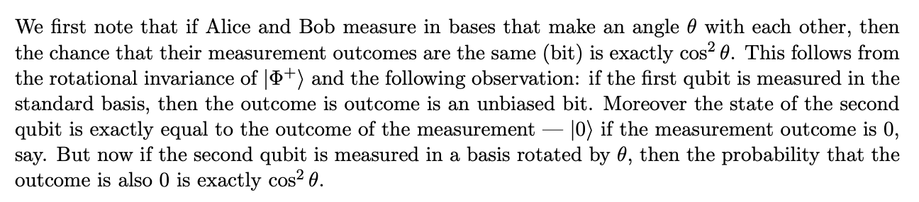
But we get \(\cos^2 \frac{\theta}{2}\). What gives? The answer to the conundrum which bothered me for many days and weeks is that the \(\theta\) used in the lecture note above is different from the \(\theta\) we are using i.e., the same symbol \(\theta\) is being used to denote different angles and creating confusion. The \(\theta\) in the lecture note above is the angle by which the 2-D basis vectors are rotated in Hilbert space. Whereas our \(\theta\) is the angle by which the Stern-Gerlach magnets are rotated in real 3D space. The two are related by factor of two which is evident when you refer the formula for the eigenspinors in this same article later on and is also called out in this article here:

For reference, here is another lecture note (and discussed in very next section of this article) which also gives \(\cos^2 \frac{\theta}{2}\) as answer.
Of the 4 bell states, the spin-singlet state also denoted as \(\Psi^-\) is the only state that is invariant to any unitary transform. All other states are invariant only to rotations. Again, read this article which explains it.
Measuring single qubit in two different bases
In this video and lecture note Umesh Vazirani considers the problem of measuring a single qubit in two different bases and calculating the probability that the qubit is in the same state in both the bases. The problem can be equivalently stated as measuring the spin of an electron - first through a detector (SG magnet) oriented along \(\hat{n}\) and then through a detector oriented along \(\hat{m}\). What is the probability that the second detector gives same spin as the first detector? The problem is same as the entangled 2 qubit system we just discussed once the first qubit has been measured. He claims following formula:
but I think this formula is incorrect in general. It only holds when \(\hat{n} = \hat{z}\). In practice this is always the case because when the experiment is performed in practice, the orientation of the first magnet is used to establish and define the \(\hat{z}\) direction. Let’s see why I think the formula is incorrect in general.
Our goal is to calculate \(P(|\hat{n} + \rangle \rightarrow |\hat{m} + \rangle)\). So we start with the wavefunction in the quantum state \(|\Psi\rangle = |\hat{n} + \rangle\) and \(P(|\hat{n} + \rangle \rightarrow |\hat{m} + \rangle)\) is simply the probability that the wavefunction will collapse to \(|\hat{m} + \rangle\) when it passes through the second magnet. To calculate this we need to express \(|\hat{n} + \rangle\) in terms of the orthonormal basis formed by \(|\hat{m} + \rangle\) and \(|\hat{m} - \rangle\) i.e.,
and then our answer is simply \(|\alpha|^2\). So how to do it?
-
First, we need to find the \(2 \times 1\) vector corresponding to \(|\hat{n} + \rangle\).
-
Then, we need to find the \(2 \times 1\) vectors corresponding to \(|\hat{m} + \rangle\) and \(|\hat{m} - \rangle\).
-
The rest is basic linear algebra you learned in undergrad classes.
Now step 1 is nothing but finding eigenvectors of \(S(\hat{n})\) - the matrix used to measure spin in the \(\hat{n}\) direction. We can get this from wikipedia:
as exercise it can be shown that the vectors above can be written in following equivalent form (see the lecture note and wikipedia for comparison; wikipedia calls these eigenspinors):
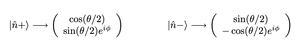
where \((\theta, \phi)\) are the spherical coordinates of \(\hat{n}\) i.e.,:
If we substitute \(n\) with \(m\) we will get \(|\hat{m} + \rangle\) and \(|\hat{m} - \rangle\). Let \(|\hat{m} + \rangle = \textbf{r}_1\) and \(|\hat{m} - \rangle = \textbf{r}_2\). Then \(\alpha\) is nothing but inner product of \(\textbf{r}_1\) and \(\textbf{q}_1\). Let’s calculate it:
Finally remember what we want is \(|\alpha|^2\). That will give \(P(|\hat{n} + \rangle \rightarrow |\hat{m} + \rangle)\). I don’t think the expression for \(\alpha\) above can be simplified to give:
If \(n_x = n_y = 0\) however, then:
and
In the lecture note he is trying to derive the fact that measuring spin along \(\hat{n}\) amounts to expressing the wavefunction in the eigenbasis formed by the eigenvectors of \(S(\hat{n})\) whereas in above we have taken it as an a-priori assumption or rule. The lecture note starts with \(P(|\hat{n}\rangle \rightarrow |\hat{m}\rangle) = \frac{1}{2} \left( 1 + \hat{n} \cdot \hat{m} \right)\) as a experimental fact, and derives \(S(\hat{n})\) from it whereas we start with \(S(\hat{n})\) and try to derive \(P(|\hat{n}\rangle \rightarrow |\hat{m}\rangle) = \frac{1}{2} \left( 1 + \hat{n} \cdot \hat{m} \right)\) from it. The lecture note develops a theory to explain the experiment whereas we start with a theory and predict experimental outcome from it.