Understanding how quantum annealing can be used to solve the QUBO problem

Preface: defining the problem

Recently I had a chance to try out D-Wave’s quantum computer. Reading their documentation, it seems this device can only do one thing which is to find the \(x\) that minimizes \(x^T Q x\) where \(x\) is a \(n\) length vector of \(0\)s and \(1\)s and \(Q\) is a symmetrical \(n \times n\) matrix. This problem is also known as Quadratic Unconstrained Binary Optimization or QUBO. Ok, no problem.

Then I read that this device uses (and works by doing) quantum annealing (QA). Now the problem:

I can find no book or reference showing that how these two things are related. How will doing QA solve a QUBO?

Wikipedia’s page on QA says:

The transverse field is finally switched off, and the system is expected to have reached the ground state of the classical Ising model that corresponds to the solution to the original optimization problem

But how? where is the proof? QM tells us that the ground-state is given by the eigenvector corresponding to lowest eigenvalue of the Hamiltonian \(H\). How is finding the minimum of \(x^T Q x\) (P1) equivalent to finding the (lowest eigenvalued) eigenvector of a matrix \(H\) (P2)? And if so, what is relation between \(Q\) and \(H\)? If P1 and P2 were same how come books on quadratic programming or wikipedia make no note of it?

I actually asked this on Stack Overflow to which the response (answer) was that consider \(Q = H\) and a proof minimizing \(x^T H x\) copied below under terms of CC BY-SA license:

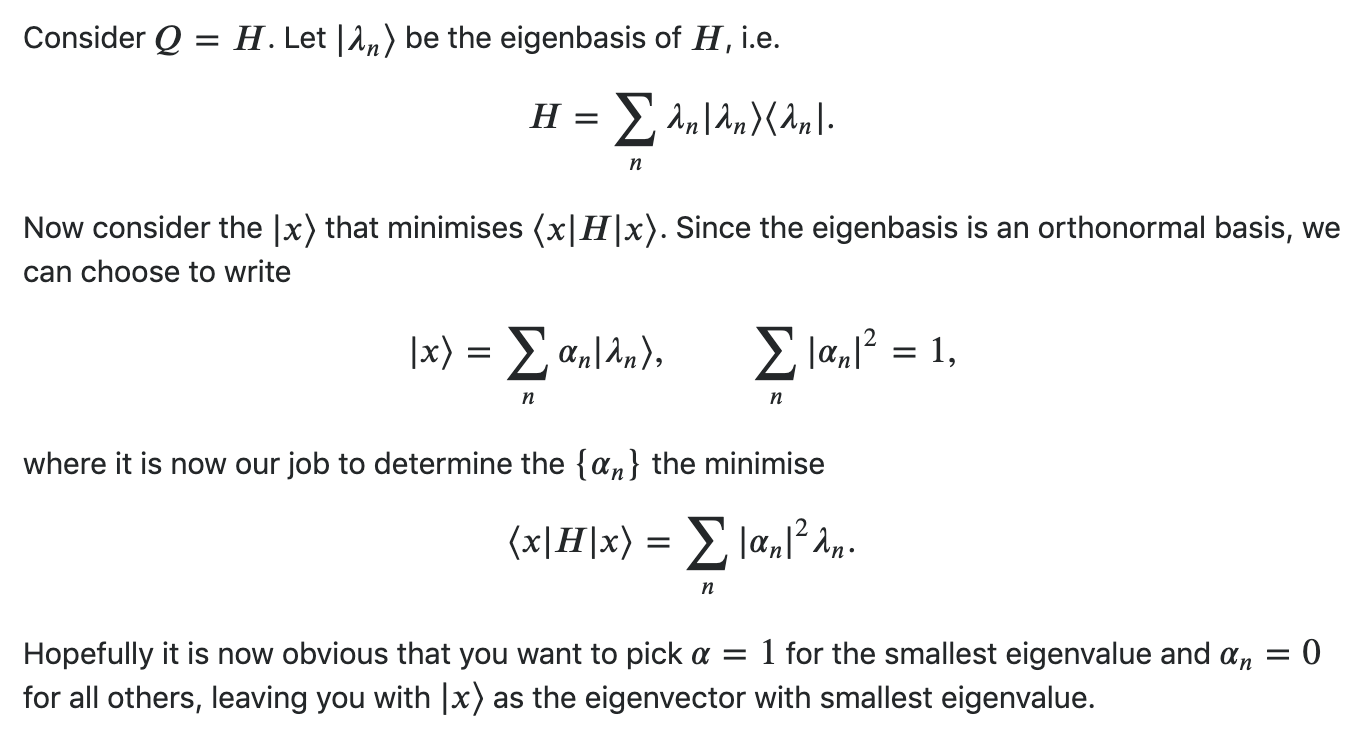
There are many problems with this answer:

The \(x\) in \(\langle x | H | x \rangle\) is a unit-length vector but the \(x\) in QUBO is not a unit-length vector. Its length can be \(0\) or more than \(1\).
The \(x\) in the answer is a vector of continuous complex variables whereas the \(x\) in QUBO contains only \(0\)s and \(1\)s.
The \(x\) in the answer is the wave function and so its length is actually \(2^n\)! Similarly, shouldn’t the Hamiltonian \(H\) be a \(2^n \times 2^n\) matrix whereas \(Q\) is \(n \times n\)?

In other words, the answer is unfortunately completely incorrect (no offense to the person who answered it - s/he is actually the top ranked user on Quantum Computing Stack Exchange). When I tried to point out these things, Stack Overflow users (many of them with \(>10\)k reputation I believe) downvoted my question and even voted to close it. The question kept bothering me though. The best I could grasp is that we use QA to minimize \(\langle \Psi | H | \Psi \rangle\) for some \(H\) - what \(H\) is continued to be unclear - make an observation (measurement) and map the result to the \(x\) of the original QUBO problem. But how does that minimize \(x^T Q x\) is a mystery until finally I got it one morning as I was getting ready to go to work…

How it works

The Ising Hamiltonian \(H\) can be seen in books or papers as defined like this:

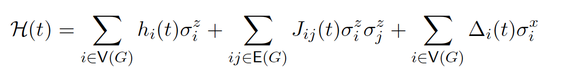
The term we need to concern ourselves with is the final Hamiltonian:

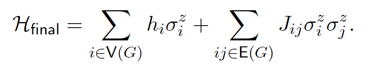
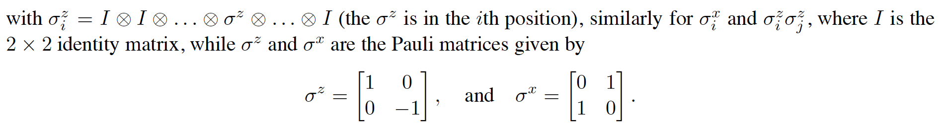
What the heck does \(\sigma_i^z\) even mean? No book will tell you that. That is why we need to go to a school where we can ask questions to a real professor. The only place where I could find an explanation was this paper (which I found as I was writing this article and after having worked out the solution myself) where he explains that:

taking an example \(n=3\), what the equation is saying is really this:

\[\begin{align} \begin{split} H & = h_1 Z \otimes I \otimes I \\ & + h_2 I \otimes Z \otimes I \\ & + h_3 I \otimes I \otimes Z \\ & + J_{12} Z \otimes Z \otimes I \\ & + J_{13} Z \otimes I \otimes Z \\ & + J_{23} I \otimes Z \otimes Z \\ \end{split} \end{align}\]

where I use \(Z\) for the \(2 \times 2\) Pauli \(\sigma^z\) matrix. We can see that \(H\) is a \(2^3 \times 2^3\) matrix. What are the eigenvalues of \(H\)? The eigenvalues of \(Z\) are \(\{-1, +1\}\) and \(I\) has only one eigenvalue namely \(1\). We use following three properties which play a key role:

Property 1 The eigenvalues of tensor product of matrices are equal to product of constituent eigenvalues i.e.

\[\begin{equation} \textrm{eig}(A \otimes B) = \textrm{eig}(A) \times \textrm{eig}(B) \end{equation}\]

refer some book on Linear Algebra if you need. The other key fact is this

Property 2 The eigenvectors of tensor product of matrices are equal to tensor product of constituent eigenvectors i.e.

\[\begin{equation} \textrm{eigvec}(A \otimes B) = \textrm{eigvec}(A) \otimes \textrm{eigvec}(B) \end{equation}\]

this is related to Property 1 and same proof applies.

Property 3 If \(A\) and \(B\) are two matrices and \(C\) is the sum of \(A\) and \(B\), then in general the eigenvalues of \(C\) are not equal to the sum of eigenvalues of \(A\) and \(B\), but if \(A\) and \(B\) have the same eigenvectors, then the eigenvalues do add up! In that case:

\[\begin{equation} \textrm{eig}(A + B) = \textrm{eig}(A) + \textrm{eig}(B) \textrm{if A and B have same eigenvectors} \end{equation}\]

Now the eigenvectors of \(Z\) are \(|0\rangle = (1,0)^T\) and \(|1\rangle = (0,1)^T\). Any vector \(v\) is an eigenvector of \(I\) but to choose a basis, we choose the same eigenvectors \((1,0)^T\) and \((0,1)^T\) for \(I\) as well. With this we can write \(H\) as:

\[\begin{equation} H = h_1 M_1 + h_2 M_2 + h_3 M_3 + J_{12} M_4 + J_{13} M_5 + J_{23} M_6 \end{equation}\]

Let’s take \(M_1 = Z \otimes I \otimes I\). By Property 1 the eigenvalues of \(M_1\) are given by \(\textrm{eig}(Z) \times \textrm{eig}(I) \times \textrm{eig}(I)\). This translates to only \(2\) distinct eigenvalues which are \(\{-1,+1\}\). Similarly, \(M_2, M_3, M_4, M_5, M_6\) all share the same set of only \(2\) distinct eigenvalues \(\{-1,+1\}\).

What are the eigenvectors of \(M_1\)? By Property 2 they are \(\textrm{eigvec}(Z) \otimes \textrm{eigvec}(I) \otimes \textrm{eigvec}(I)\). This gives us following 8 vectors (enumerating all combinations):

\[\begin{align} \begin{split} |0\rangle \otimes |0\rangle \otimes |0\rangle & = |000\rangle \\ |0\rangle \otimes |0\rangle \otimes |1\rangle & = |001\rangle \\ |0\rangle \otimes |1\rangle \otimes |0\rangle & = |010\rangle \\ |0\rangle \otimes |1\rangle \otimes |1\rangle & = |011\rangle \\ |1\rangle \otimes |0\rangle \otimes |0\rangle & = |100\rangle \\ |1\rangle \otimes |0\rangle \otimes |1\rangle & = |101\rangle \\ |1\rangle \otimes |1\rangle \otimes |0\rangle & = |110\rangle \\ |1\rangle \otimes |1\rangle \otimes |1\rangle & = |111\rangle \\ \end{split} \end{align}\]

These are nothing but the computational basis vectors in \(2^3\)-D space. By same analysis we can show \(M_2, M_3, M_4, M_5, M_6\) all share the same set of eigenvectors above.

So now we have shown \(M_1, M_2, M_3, M_4, M_5, M_6\) all have same eigenvalues and eigenvectors. Applying Property 3, we may be tempted to infer the eigenvalues of \(H\) as:

\[\begin{equation} \textrm{eig}(H) = h_1 b_1 + h_2 b_2 + h_3 b_3 + J_{12} b_4 + J_{13} b_5 + J_{23} b_6 \textrm{(wrong)} \end{equation}\]

where \(b_i\) are independent variables having values \(\{-1,+1\}\) but this is wrong. For one this gives us \(2^6\) combinations of \(b_i\)'s whereas \(H\) should have \(2^3\) eigenvalues. The correct way to calculate the eigenvalues of \(H\) is to apply \(H\) to the eigenvectors of \(M_1, M_2, M_3, M_4, M_5, M_6\) we calculated above. For example:

\[\begin{align} H|101\rangle & = h_1 M_1 |101\rangle + h_2 M_2 |101\rangle + h_3 M_3 |101\rangle + J_{12} M_4 |101\rangle + J_{13} M_5 |101\rangle + J_{23} M_6 |101\rangle \end{align}\]

where:

\[\begin{align} \begin{split} M_1 |101\rangle & = (Z \otimes I \otimes I) (|1\rangle \otimes |0\rangle \otimes |1\rangle) \\ & = Z |1\rangle \otimes I |0\rangle \otimes I |1\rangle \; \; \textrm{since} (A \otimes B) (C \otimes D) = (AC \otimes BD) \\ & = -|1\rangle \otimes |0\rangle \otimes |1\rangle \\ & = -|101\rangle \end{split} \end{align}\]

Similarly we have to do for \(M_2, M_3, M_4, M_5, M_6\). In general given the eigenvector \(|x_1 x_2 x_3 \rangle\) (\(x_i \in \{0,1\}\)):

\[\begin{align} \begin{split} M_1 |x_1 x_2 x_3 \rangle & = h_1 (Z \otimes I \otimes I) (|x_1\rangle \otimes |x_2\rangle \otimes |x_3\rangle) \\ & = h_1 Z |x_1\rangle \otimes I |x_2\rangle \otimes I |x_3\rangle \\ & = h_1 (-1)^{x_1}|x_1\rangle \otimes |x_2\rangle \otimes |x_3\rangle \\ & = h_1 (-1)^{x_1}|x_1 x_2 x_3\rangle \end{split} \end{align}\]

\[\begin{align} \begin{split} M_2 |x_1 x_2 x_3 \rangle & = h_2 (I \otimes Z \otimes I) (|x_1\rangle \otimes |x_2\rangle \otimes |x_3\rangle) \\ & = h_2 I |x_1\rangle \otimes Z |x_2\rangle \otimes I |x_3\rangle \\ & = h_2 |x_1\rangle \otimes (-1)^{x_2}|x_2\rangle \otimes |x_3\rangle \\ & = h_2 (-1)^{x_2}|x_1 x_2 x_3\rangle \end{split} \end{align}\]

\[\begin{align} \begin{split} M_3 |x_1 x_2 x_3 \rangle & = h_3 (I \otimes I \otimes Z) (|x_1\rangle \otimes |x_2\rangle \otimes |x_3\rangle) \\ & = h_3 I |x_1\rangle \otimes I |x_2\rangle \otimes Z |x_3\rangle \\ & = h_3 |x_1\rangle \otimes |x_2\rangle \otimes (-1)^{x_3}|x_3\rangle \\ & = h_3 (-1)^{x_3}|x_1 x_2 x_3\rangle \end{split} \end{align}\]

\[\begin{align} \begin{split} M_4 |x_1 x_2 x_3 \rangle & = J_{12} (Z \otimes Z \otimes I) (|x_1\rangle \otimes |x_2\rangle \otimes |x_3\rangle) \\ & = J_{12} Z |x_1\rangle \otimes Z |x_2\rangle \otimes I |x_3\rangle \\ & = J_{12} (-1)^{x_1} |x_1\rangle \otimes (-1)^{x_2} |x_2\rangle \otimes |x_3\rangle \\ & = J_{12} (-1)^{x_1 + x_2} |x_1 x_2 x_3\rangle \end{split} \end{align}\]

\[\begin{align} \begin{split} M_5 |x_1 x_2 x_3 \rangle & = J_{13} (Z \otimes I \otimes Z) (|x_1\rangle \otimes |x_2\rangle \otimes |x_3\rangle) \\ & = J_{13} Z |x_1\rangle \otimes I |x_2\rangle \otimes Z |x_3\rangle \\ & = J_{13} (-1)^{x_1} |x_1\rangle \otimes |x_2\rangle \otimes (-1)^{x_3}|x_3\rangle \\ & = J_{13} (-1)^{x_1 + x_3} |x_1 x_2 x_3\rangle \end{split} \end{align}\]

\[\begin{align} \begin{split} M_6 |x_1 x_2 x_3 \rangle & = J_{23} (I \otimes Z \otimes Z) (|x_1\rangle \otimes |x_2\rangle \otimes |x_3\rangle) \\ & = J_{23} I |x_1\rangle \otimes Z |x_2\rangle \otimes Z |x_3\rangle \\ & = J_{23} |x_1\rangle \otimes (-1)^{x_2} |x_2\rangle \otimes (-1)^{x_3}|x_3\rangle \\ & = J_{23} (-1)^{x_2 + x_3} |x_1 x_2 x_3\rangle \end{split} \end{align}\]

Introduce following variables: \(s_i = (-1)^{x_i}\) for \(i \in \{1,2,3\}\). Then we can write \(H|x_1 x_2 x_3 \rangle\) as:

\[\begin{equation} H|x_1 x_2 x_3 \rangle = (h_1 s_1 + h_2 s_2 + h_3 s_3 + J_{12} s_1 s_2 + J_{13} s_1 s_3 + J_{23} s_2 s_3) |x_1 x_2 x_3 \rangle \end{equation}\]

and so \(|x_1 x_2 x_3 \rangle\) is an eigenvector of \(H\) and the eigenvalues (allowed energy levels) of \(H\) are in fact given by:

\[\begin{align} \begin{split} E & = h_1 s_1 + h_2 s_2 + h_3 s_3 + J_{12} s_1 s_2 + J_{13} s_1 s_3 + J_{23} s_2 s_3 \end{split} \end{align}\]

where \(s_1, s_2, s_3\) are binary variables taking on values \(\{-1, +1\}\) (the eigenvalues of \(Z\)). E.g., the combination \((-1,+1,-1)\) of \((s_1, s_2, s_3)\) gives one possible value of \(E\). This is nothing but the QUBO cost function. The ground-state is the state that minimizes \(E\) and if we measure the values of the spins (qubits) in the ground state (measurement of a qubit will yield \(-1\) or \(+1\)) we will find the vector \(x\) that minimizes the QUBO cost function. So this is how it works. If you do the math, it turns out the (final) Ising Hamiltonian is actually a diagonal matrix containing the energy values \(E\) on its diagonal. All the off-diagonal elements are \(0\). This is just another way of saying that the eigenvectors of \(H\) are the same as the vectors of the computational basis. Going back to OP, there is a trivial relation (equivalence) between P1 (minimize \(x^T Q x\)) and P2 (eigendecomposition of some \(H\)) which is simply this: calculate all \(2^n\) values of \(x^T Q x\). Put them on the diagonal of a \(2^n \times 2^n\) matrix. That matrix is \(H\). This relation is not very useful for classical optimization algorithms and that’s why there is no mention of it in books on quadratic programming.

This also explains why the D-Wave computer is a special purpose computer because its Hamiltonian is constrained to be an Ising Hamiltonian in a transverse field.