Understanding Quantum Key Distribution (QKD)

Preface from wikipedia: Quantum key distribution (QKD) is a secure communication method which implements a cryptographic protocol involving components of quantum mechanics. It enables two parties to produce a shared random secret key known only to them, which can then be used to encrypt and decrypt messages. It is often incorrectly called quantum cryptography, as it is the best-known example of a quantum cryptographic task.

IBM has a good tutorial on it that explains it using the BB84 protocol. Read it if you like. Here I try to explain QKD in my own words.

QKD works by encoding a classical bit string as a string of quantum states. The B92 protocol for example encodes \(0\) as \(|0\rangle\) and \(1\) as \(| + \rangle\). If you don’t understand what \(|0\rangle\) and \(| + \rangle\) mean, stop reading and come back when you have understood the basics. So if Alice has a classical binary string \(1000101011010100\), this will get encoded as \(\Psi = | + 000+0+0++0+0+00\rangle\) and sent over a channel over which Eve might be listening. In physical terms what happens is that \(16\) photons will be sent over an optical fiber. The photons corresponding to \(0\) will have \(0^{\circ}\) polarization and the photons corresponding to \(1\) will have \(45^{\circ}\) polarization. There is no entanglement between the photons.

You might be thinking how stupid is that. We already know the rule for encoding the binary string - its pretty simple. We can just decode the message \(|\Psi\rangle\) using that rule and get back the original string of bits. Here is where QM comes in. In QM it is impossible to fully know the complete state of a quantum system (Heisenberg’s uncertainty principle). Thus Eve has no instrument (think wireshark if you will) that can take input \(|\Psi\rangle\) (\(|\Psi\rangle\) is nothing but the \(16\) photons we transmitted) and give \(| + 000+0+0++0+0+00\rangle\) as a readout which she can then decode as \(1000101011010100\). ^[1] All she can do is two things:

Apply a unitary evolution to \(|\Psi\rangle\) to yield another quantum state \(|\Phi\rangle\)
Or, make a measurement. Making a measurement requires choosing a basis first of all. Then when a measurement is made, the quantum state will collapse to one of the basis vectors (very much like we project vectors to a basis in Linear Algebra classes) with a probability given by the Born rule. In the photon example, measurement corresponds to measuring the polarization of the photons. For this, we have to choose two axes along which we will measure the polarization. This corresponds to fixing the basis.

The measurement destroys the original state unless the state happened to be one of the basis vectors (this follows directly from Linear Algebra). Some examples might help clear this up. Consider the state \(|0\rangle\). This corresponds to the vector \((1,0)^T\) in Hilbert space. When measured in the \(Z\) basis which I call the canonical (native) basis (it is the canonical or native basis because its made up of the basis vectors \((1,0)^T\) and \((0,1)^T\)), the state remains undisturbed and we consider this as measuring \(0\). But look what happens if \(| + \rangle\) were measured in this basis. \(|+ \rangle\) stands for \((1, 1)^T\) (I have dropped the \(\frac{1}{\sqrt{2}}\) normalization constant for convenience). Projecting (measuring is the better word) \((1, 1)^T\) onto the canonical basis gives \((1, 0)^T\) or \((0, 1)^T\) with equal probability. The original state is destroyed and this lies at the heart of QKD. The state that Bob will get will now be different from the state Alice had sent and they will be able to detect this and infer that someone had eavesdropped the channel.

Let’s recap. Imagine Alice wishes to communicate a single bit of classical information. It has two states \(0\) and \(1\) and when its transmitted its transmitted as a quantum state \(|0\rangle\) or \(|+ \rangle\) respectively. Assume there is no eavesdropping for now. If Bob chooses to measure the received signal in \(Z\) basis, he gets \(0\) for \(|0\rangle\) but \(0\) or \(1\) with equal probability for \(|+\rangle\). So if Bob measures \(0\), he can’t be sure whether Alice sent \(0\) or \(1\). But if he measures \(1\), he can be sure that Alice sent \(1\) (it might be more appropriate to say that Alice meant to communicate a \(1\). I use colloquial language for ease of understanding).

Suppose Bob was instead measuring in the \(X\) basis - this basis has the basis vectors \((1,1)^T\) and \((-1,1)^T\). In this basis \(|0\rangle\) will appear (i.e., will be measured) as \(0\) or \(1\) with equal probability but \(|+ \rangle\) will appear as \(0\) with \(100\%\) probability as \(|+ \rangle\) is a basis vector of the \(X\) basis. So in this basis if Bob measures \(0\), again he can’t be sure whether Alice sent a \(0\) or a \(1\), but if he measures \(1\), he can be sure that a \(0\) was sent.

Here is the summary in absence of noise or eavesdropping:

Table 1. B92 Protocol
Alice’s bit (\(a\))	\(\|\Psi \rangle = f(a)\)	Bob’s basis	Bob’s measurement
\(0\)	\(\|0 \rangle\)	\(Z\)	\(0\)
\(1\)	\(\|+ \rangle\)	\(Z\)	\(0\) or \(1\) with equal prob.
\(0\)	\(\|0 \rangle\)	\(X\)	\(0\) or \(1\) with equal prob.
\(1\)	\(\|+ \rangle\)	\(X\)	\(0\)

Now, to understand the B92 protocol, let’s put it into action. Let’s see what happens when we take the happy path, when there is no noise in the channel (equivalently Eve is not eavesdropping)

Step 1: Alice generates a binary string, encodes it and transmits it

We covered this step before. Binary string = \(a = 1000101011010100\), message = \(\Psi = |+ 000+0+0++0+0+00\rangle\). Remember Alice keeps \(a\). She does not send it.

Step 2: Bob decodes the message using a random basis he chooses

Bob randomly and independently decodes (measures) each qubit using either \(X\) or \(Z\) basis. Suppose he decided to use \(ZZXZXXXZXZXXXXXX\) for his measurements. Applying Table 1, Bob will get

a	1	0	0	0	1	0	1	0	1	1	0	1	0	1	0	0
basis	Z	Z	X	Z	X	X	X	Z	X	Z	X	X	X	X	X	X
observation	?	0	?	0	0	?	0	0	0	?	?	0	?	0	?	?

The ? are the qubits which he will randomly measure as \(0\) or \(1\) with equal probability. Remember that Bob does not have access to the top row in above table. It is there for illustration purposes only. To keep going, suppose he measures (in below I delete the top row from previous table to show Bob’s view):

Z	Z	X	Z	X	X	X	Z	X	Z	X	X	X	X	X	X
0	0	1	0	0	1	0	0	0	0	1	0	1	0	1	1

Step 3: We check if message has been compromised

To do this, take a look at the qubits that were measured as \(1\). For example, in above the rightmost qubit is \(1\) and the \(X\) basis was used to measure it. From preceeding discussion we learned that when \(X\) basis is used for measurement and a \(1\) observation is made, Bob can be certain that a \(0\) was "sent" by Alice. i.e., in below:

basis	Z	Z	X	Z	X	X	X	Z	X	Z	X	X	X	X	X	X
measurement	0	0	1	0	0	1	0	0	0	0	1	0	1	0	1	1

Wherever there is a \(0\), Bob cannot say what Alice holds at that position, but wherever there is a \(1\) Bob can be confident what Alice holds depending on the basis (\(X\) or \(Z\)).

So Bob will ask Alice, is the rightmost bit in \(a\) a \(0\)? If Alice answers no Bob knows that channel has been compromised (note this assumes Alice’s answer reaches Bob unmodified). If Alice answers yes there is now a non-zero probability \(p\) that no eavesdropping has occured. This probability \(p\) increases as more and more bits where we observe \(1s\) are compared. In above we got total \(6\) \(1s\). We can choose to use \(3\) for testing if channel has not been compromised. If answer is affirmative then, the remaining \(3\) can be used to share a private key between Alice and Bob.

And this is how B92 protocol works.

In some sense it is even more simpler (elegant) than the BB84 protocol because here the encoding of classical bits to qubits is well-known in advance. It is a static rule and not dependent upon another random string generated at runtime as in case of BB84.

At heart of QKD is the lemma that it is impossible to distinguish two non-orthogonal quantum states without introducing a disturbance to either of them. And the no-cloning theorem which guarantees that it is impossible to clone or copy a quantum state. What QM taketh (impossible to fully know the complete state of a system) it giveth it away (a provably secure means of private key generation).

A great simulation of the protocol can be found here

It is possible to write a python program to simulate B92. The main function looks like this:

eavesdrop = np.random.choice([True, False], size=N_trials)
for i in range(0, N_trials):
    (key, is_compromised) = perform_b92_experiment(N_bits, N_test, eavesdrop[i])
    if eavesdrop[i]:
        num_positive += 1
        if is_compromised:
            true_positive += 1
        else:
            false_negative += 1 # Alice and Bob think the key is not compromised when in fact it has been compromised
    else:
        num_negative += 1
        if is_compromised:
            false_positive += 1 # Alice and Bob think the key is compromised when in fact it hasn't been compromised. This cannot happen with B92 protocol
        else:
            true_negative += 1
            key_length.append(len(key)) # length of the shared key established between alice and bob

The perform_b92_experiment takes input 3 parameters:

N_bits: The number of bits in \(a\), Alice’s binary string
N_test: The (maximum) number of bits that will be used for testing whether the message or channel has been compromised by an eavesdropper
eavesdrop: Whether to eavesdrop on the signal or not

and returns 2 outputs:

key: The shared secret
is_compromised: Whether the protocol determines that the channel has been compromised

Filling out perform_b92_experiment is left as an exercise. When I performed the experiment \(1000\) times with N_bits=160 and N_test=10, this is what I found:

total trials =  1000
num positive =  507
num_negative =  493
true positive =  499
true negative =  493
false positive =  0
false negative =  8
Confusion Matrix
0.9842209072978304   0.015779092702169626
0.0   1.0
avg. key length =  30.352941176470587

What do you get?

I then decided to try out the BB84 protocol. For BB84, this is what I got with identical settings:

total trials =  1000
num positive =  493
num_negative =  507
true positive =  466
true negative =  507
false positive =  0
false negative =  27
Confusion Matrix
0.9452332657200812   0.05476673427991886
0.0   1.0
avg. key length =  70.23668639053254

so we can see it has a higher error rate than B92. On the other hand the avg. key length is more than double than in case of B92. In general, IBM’s tutorial for BB84 determines its error rate as \(p(\textrm{undetected}) = 0.75^t\) where \(t\) is the number of bits used for testing. I initially thought the error rate for B92 will be the same but computer simulation says otherwise. Can we figure out error rate for B92?

B92 Error Analysis

First, note that the protocol cannot give any false positive. false positive = protocol determines channel has been spoofed when in fact it hasn’t. This cannot happen. And that is true for BB84 as well. So the error rate is the rate of false negative. false negative = Alice and Bob think the channel is not compromised when in fact it has been compromised. How can we calculate it? Below graph of possible outcomes provides the answer:

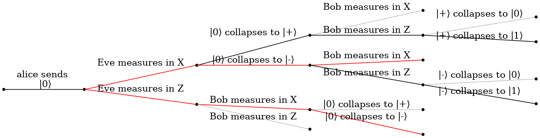
It shows the case when Alice has a \(0\) bit to send to Bob. The only way this can go undetected in the presence of eavesdropping by Eve is shown by the two red paths and the probability is given by:

\[\begin{align} \begin{split} p(\textrm{false negative}) & = p(\textrm{Eve decides to measure in } Z) \\ & \times p(\textrm{Bob decides to measure in } X) \\ & \times p(\textrm{Bob measures } 1) \\ & + p(\textrm{Eve decides to measure in } X) \\ & \times p(|0\rangle \textrm{ collapses to } |- \rangle \textrm{ after Eve's measurement}) \\ & \times p(\textrm{Bob decides to measure in } X) \\ & = \frac{1}{2} \cdot \frac{1}{2} \cdot \frac{1}{2} + \frac{1}{2} \cdot \frac{1}{2} \cdot \frac{1}{2} \\ & = \frac{1}{4} (\textrm{incorrect}) \end{split} \end{align}\]

Note that when Bob receives a \(|-\rangle\) which is an invalid state since Alice encodes \(0\) as \(|0\rangle\) and \(1\) as \(|+ \rangle\), there is no way for him to know that he has received a \(|-\rangle\). All he can do is measure. The above formula is not the correct answer actually (and it took me a while to figure out). My simulations were giving \(p(\textrm{false negative}) = 0.66\) and I just couldn’t figure out whether the simulations were incorrect or the analysis was incorrect. As it happens, I kept pondering the whole day and could not determine which one is correct. Then next morning when I woke up, I realized. This happens very frequently. I think the brain does an awful amount of work during sleeping but that is tpoic for another post. It turns out the analysis is incorrect, or rather incomplete. Bob performs a test only when the measured qubit is a \(1\). We need to factor that in above by dividing \(0.25\) by the probability of observing a \(1\). That means we need to exclude the paths colored in gray - those are the paths that end up with a \(0\) measurement by Bob. The probability of observing a \(1\) is given by:

\[\begin{align} \begin{split} p(\textrm{1}) & = \frac{1}{4} + \frac{1}{16} + \frac{1}{16} \\ & = \frac{3}{8} \end{split} \end{align}\]

Note very carefully that the probability of Bob observing a \(1\) changes if Eve is listening on the channel. Without Eve listening, this probability is \(0.25\) following the arguments earlier in the article (refer Table 1). This provides us another way to test if channel has been compromised. The correct formula for \(p(\textrm{false negative})\) is:

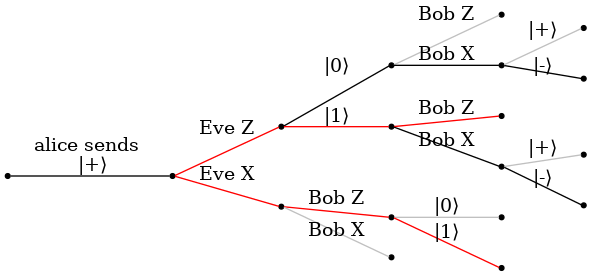
\[\begin{align} \begin{split} p(\textrm{false negative}) & = \frac{\frac{1}{4}}{\frac{3}{8}} \\ & = \frac{2}{3} (\textrm{correct}) \end{split} \end{align}\]

There is a symmetric case when Alice has a \(1\) bit to send to Bob. It is shown below for completeness:

Both cases have equal chance to happen so the overall error rate remains \(\frac{2}{3}\). So if we test using \(t\) bits, the error rate of B92 protocol is given by (deserves an equation of its own):

\[\begin{equation} p(\textrm{false negative}) = \left( \frac{2}{3} \right) ^ t \end{equation}\]

Note carefully that above analysis (as well as the simulations I did) assumes Eve is also measuring in either \(Z\) or \(X\) with equal prob. This cannot be the case necessarily. In general Eve could measure in a basis whose vectors form an angle \(\theta\) with \(Z\).

We can see that B92’s error rate is slightly better than BB84’s error rate. The BB84 protocol requires \(1.4\) times \(\left( \frac{\log(0.66)}{\log(0.75)} \right)\) as many bits as B92 to achieve the same error rate. The improved error rate comes at the cost of shorter key length as I have seen in my simulations.

Average Key Length

Can we derive formulae for the average key length of the two protocols? Yes we can. In case of BB84, the number of eligible bits is given by number of times the chosen bases between Alice and Bob match. This has a \(50\%\) of chance of happening for each qubit independent of others. And so if \(n\) is the number of total qubits transmitted (also equal to length of Alice’s binary string):

\[\begin{equation} \textrm{BB84: } \textrm{avg. key length} + \textrm{number of bits used for testing} = 0.5n \end{equation}\]

In case of B92, bits measured as \(0\) by Bob are discarded and \(1\) bits are kept. The probability of observing a \(1\) by Bob is \(0.25\) in absence of noise (eavesdropping). And so the corresponding formula in case of B92 is:

\[\begin{equation} \textrm{B92: } \textrm{avg. key length} + \textrm{number of bits used for testing} = 0.25n \end{equation}\]

Now, given a desired error rate \(e\), and average key length \(l\), what should be \(n\) for the two protocols? Let’s do it for BB84 first.

\[\begin{split} \begin{align} \textrm{BB84: } l + \frac{\log(e)}{\log(0.75)} = 0.5n \end{align} \end{split}\]

and so,

\[\begin{split} \begin{align} \textrm{BB84: } n & = 2 \left( l + \frac{\log(e)}{\log(0.75)} \right) \\ & \approx 2 l + 7.0 \log{\frac{1}{e}} \end{align} \end{split}\]

In case of B92:

\[\begin{split} \begin{align} \textrm{B92: } l + \frac{\log(e)}{\log(0.66)} = 0.25n \end{align} \end{split}\]

and so,

\[\begin{split} \begin{align} \textrm{B92: } n & = 4 \left( l + \frac{\log(e)}{\log(0.66)} \right) \\ & \approx 4 l + 9.9 \log{\frac{1}{e}} \end{align} \end{split}\]

The \(\log\) is w.r.t. natural base in above equations (i.e., \(\log(2.718281828459) = 1\)). Below are some numerical calculations with \(l = 32\) and varying \(e\) for the two protocols:

Table 2. BB84 vs B92: number of qubits required to get a desired error rate and average key length
e	BB84	B92
0.01	96	173
0.001	112	196
0.0001	128	219
0.00001	144	242
0.000001	160	264
\(10^{-30}\)	544	809

1. In physical terms given a photon, there is no way to know how Alice polarized it. All we can do is measure the polarization in some basis. That gives us the component of polarization along that basis and in the process the original state is destroyed.